Optimization of sub-multihomogeneous functions

The connection between eigenvalue problems and constrained optimization is relatively standard. For example, the singular value equations \(M y = \lambda x\), \(M^\top x = \lambda y\) of a matrix \(M\) always admit a variational characterization which connects the solutions of the constrained optimization of \(f(x,y) = x^\top M y\) to the singular values and vectors of \(M\). In particular, the constrained optimization problem

\[\begin{equation}\label{eq:matrix-variational-problem} \left\{ \begin{array}{ll} \text{max} & f(x,y) \\[.4em] \text{subject to}& \|x\|= \|y\|=1 \end{array} \right. \end{equation}\]

is given by the extreme left and right singular vectors of \(M\). Thus, while the optimization problem itself is not convex in general (for a general \(M\)), we can compute it using ideas from numerical linear algebra, in particular, numerical eigensolvers. This relatively simple connection has led to powerful numerical optimizers in recent years, see e.g. ¹ ² ³.

A simple application of Euler’s theorem shows that an analogous property holds for the more general constrained optimization problem

\[\begin{equation}\label{eq:constrained-opt} \left\{ \begin{array}{ll} \text{max}_{x\in \RR^n} & f(x^{(1)}, \dots, x^{(s)})\\ \text{subject to}& g_1(x^{(1)})=\dots=g_s(x^{(s)})=1, \end{array} \right. \end{equation}\]

where \(f\) and \(g_i\) are multihomogeneous or, more generally, sub-multihomogeneous. However, when \(f\) and \(g_i\) are not quadratic, this optimization problem can be significantly more challenging than \(\eqref{eq:matrix-variational-problem}\). As we will see, even smooth functions \(f\) and \(g_i\) may lead to NP-hard problems. However, when \(f\) and \(g_i\) are nonnegative, we can often solve \(\eqref{eq:constrained-opt}\) to an arbitrary accuracy by leveraging and extending the Perron-Frobenius theory for multihomogeneous mappings. This is a main result we will present below, in the Global optimization setting section.

Before doing this, we discuss an example which shows how the constrained optimization of homogeneous functions pops up in combinatorial optimization and has applications for example in graph clustering.

Optimization of combinatorial ratios

Consider a set of integers \(V=\{1,\dots, n\}\). A combinatorial ratio is a function \(f:2^V\to\RR\) of the form

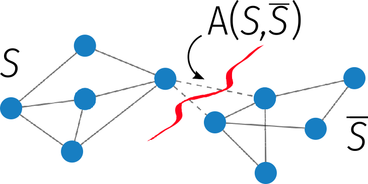
\[\begin{equation}\label{eq:general-ratio} \vartheta(S) = \frac{\alpha(S)}{\beta(S)} \end{equation}\]

where both \(\alpha\) and \(\beta\) are set functions \(\alpha,\beta:2^V\to\RR\). The optimization of this type of functions arises in many context. One example of interest to us is graph clustering. The optimization of the graph conductance is a classical and successful strategy for finding a good partition of a graph into two subsets. In this case \(V\) is the vertex set of a graph \(G=(V,E)\) with adjacency matrix \(A\) and the global minimum of

\[ \vartheta(S) = \frac{A(S,\bar S)}{\min\{\nu(S),\nu(\bar S)\}} \]

where \(\bar S = V\setminus S\) is the complement of \(S\) in \(V\), \(A(S,\bar S) = \sum_{i\in S, j\in \bar S}A_{ij}\) is the overall weight of edges going from \(S\) to \(\bar S\) and \(\nu(S)=\sum_{i\in S}\nu_i\) is the weight of the set \(S\), for some weight coefficients \(\nu_i\).

Minimizing \(\vartheta\) is in general a NP-hard problem, however a homogeneous relaxation based on the Lovasz extension of \(\alpha\) and \(\beta\) allows us to obtain arbitrarily good continuous approximation. This was first observed in ⁴ for \(1\)-homogeneous functions, but it is not difficult to extend that idea to the case of \(p\)-homogeneous ones:

Theorem. Let \(\alpha,\beta:2^V\to\RR\) be such that \(\alpha(S),\beta(S)\geq 0\) for all \(S\subseteq V\) and \(\alpha(V)=\alpha(\emptyset)=\beta(V)=\beta(\emptyset)=0\). For any \(p\geq 1\) there exist a constant \(C\) independent of \(n\) and \(p\) and homogeneous functions \(f,g:\RR^n\to\RR\) with homogeneity degree \(p\) such that, if \(\lambda\) is the solution to

\[\begin{equation}\label{eq:thm-cheeger} \lambda = \min \Big\{ f(x) \text{ such that } g(x) = 1 \Big\} \end{equation}\]

then \(\lambda \leq \min_S \vartheta(S)\leq C^{p-1} \lambda^{1/p}\). In particular, \(\lambda \xrightarrow{p\to 1} \min \vartheta\).

Both \(f\) and \(g\) in the theorem above are defined in terms of the Lovasz extension of \(\alpha\) and \(\beta\). For certain combinatorial functions this extension admits an explicit formula. For example, when tailored to the clustering problem \(\alpha(S) = A(S,\bar S)\) and \(\beta(S) =\min\{\nu(S),\nu(\bar S)\}\), the \(p\)-homogeneous functions in the theorem are

\[ f(x) = \frac 1 2 \sum_{ij}A_{ij}|x_i-x_j|^p \qquad \text{and} \qquad g(x) = \|x-\mathrm{mean}(x)\one\|_p^p\, . \]

In particular, \(f(x)\) is the energy associated to the so-called \(p\)-Laplacian on \(G\) and in fact, it is not difficult to show that for these two \(f\) and \(g\), \(\lambda\) in the theorem coincides with the smallest nonzero eigenvalue of the graph \(p\)-Laplacian, defined as

\[ L_p(x) = B\Phi(B^\top x), \qquad \Phi(x) = |x|^{p-1}\mathrm{sign}(x) \]

with \(B\) the incidence matrix of \(G\) (see the network centrality section for its definition). In particular, \(L_p\) boils down to the graph Laplacian matrix when \(p=2\) and we obtain the renowned Cheeger inequality as a corollary of the theorem above.

This observation shows that the optimization of the graph conductance can be approached via the solution of so-called nonlinear eigenvalue problems with eigenvector nonlinearities. In fact, using the Euler theorem for (multi)homogeneous functions, we can always connect the constrained optimization problem \(\eqref{eq:constrained-opt}\) with a nonlinear eigenvector problem, as we will discuss next.

Sub-multihomogeneous mappings

Our main result concerns the global solution of the constrained optimization problem \(\eqref{eq:constrained-opt}\) and holds for a family of operators that generalized the already discussed set of homogeneous mappings. This is the class of sub-multihomogeneous maps. We provide here their definition, first starting from a different characterization of the multihomogeneous ones.

A mapping \(F:\RR^n\to\RR^m\) is homogeneous with homogeneity coefficient \(p\) if \(F(\lambda x)=\lambda^p F(x)\) for all \(\lambda>0\) and \(x\succeq 0\). When \(F\) is differentiable, Euler’s theorem for homogeneous functions allows us to equivalently characterize this property in terms of the Jacobian of \(F\), which we denote by \(\partial F:\RR^n\to\RR^{m\times n}\). Precisely, we have

Theorem (Euler). Let \(F:\RR^n\to\RR^{m}\) be differentiable. Then \(F\) is homogeneous with homogeneity coefficient \(p\neq 0\) if and only if \(\partial F(x)x = p F(x)\) for all \(x\succ 0\).

This result can be extended to the multihomogeneous setting. In fact, as for homogeneous functions, multihomogeneous mappings enjoy a similar Euler-based characterization.

To fix the ideas, consider first the case of two variable sets \(x = (x^{(1)},x^{(2)})\) with \(x^{(1)}\in\RR^{n_1}\) and \(x^{(2)}\in \RR^{n_2}\) and \(n_1+n_2=n\). Let \(F= (F_1,F_2):\RR^n\to\RR^n\) be a multihomogeneous mapping with \(2\times 2\) homogeneity matrix \(\M\). In this notation, each \(F_i\) is a map from \(\RR^{n_1+n_2}\) to \(\RR^{n_i}\). Moreover, we assume

\(\partial_j = \partial_{x^{(j)}}\) denotes the partial derivative with respect to the set of variables \(x^{(j)}\)

then, for any \(x\in \RR^{n_1+n_2}\), \(\partial_j F_i(x)\) is a \(n_i\times n_j\) matrix and we can partition \(\M\), \(F\), and its Jacobian \(\partial F\) as

\[ \M = \begin{bmatrix} \M_{11} & \M_{12}\\ \M_{21} & \M_{22} \end{bmatrix} \qquad F(x) = \left[ \begin{array}{c} \begin{array}{c} \\ F_1(x)\\ \, \end{array} \\ \hline F_2(x) \end{array}\right] \qquad \partial F(x) = \left[ \begin{array}{c|c} \begin{array}{ccc} && \\ & \partial_{1}F_1(x) &\\ && \end{array} & \partial_2 F_1(x) \\ \hline \partial_1 F_2(x) & \partial_2 F_2(x) \end{array}\right] \]

If we apply the Euler’s theorem to each of the blocks individually, we obtain that the following identities

\[ \begin{cases} \partial_1 F_1(x)x^{(1)} = \M_{11} F_1(x) & \partial_2 F_1(x)x^{(2)} = \M_{12} F_1(x) \\ \partial_1 F_2(x)x^{(1)} = \M_{21} F_2(x) & \partial_2 F_2(x)x^{(2)} = \M_{22} F_2(x) \end{cases} \]

equivalently characterize \(F\) as a multihomogeneous mapping. More in general, we have

Theorem. Let \(F=(F_1,\dots,F_t):\RR^n\to\RR^m\) be differentiable. Then \(F\) is multihomogeneous of homogeneity matrix \(\M\) of size \(s\times t\) if and only if there exists a subdivision of the variable \(x\) into \(x=(x^{(1)}, \dots, x^{(s)})\) such that

\[ \partial_j F_i(x) x^{(j)} = \M_{ij} \, F_i(x) \]

for all \(i,j\) and all \(x=(x^{(1)}, \dots, x^{(s)})\succ 0\).

The theorem above fully characterizes differentiable multihomogeneous operators and, when \(F\) is order-preserving, i.e. \(F(x)\succeq 0\) when \(x\succeq 0\), it implies that \(|\partial_j F_i(x)| x^{(j)} = |\M_{ij}| \, F_i(x)\) for a multihomogeneous mapping, where absoulute values are taken entrywise.

This motivates the following

Definition. A differentiable \(F:\RR^n\to\RR^m\) is sub-multihomogeneous of homogeneity matrix \(\M\) if there exists a partition of the variable \(x\) such that

\[ |\M_{ij}| = \min\Big\{\lambda \geq 0 \, : \, |\partial_j F_i(x)| x^{(j)} \leq \lambda \, F_i(x) \Big\} \]

for all \(i,j\) and all \(x\succ 0\).

Clearly, any multihomogeneous operator is also sub-multihomogeneous, with the same homogeneity matrix.

In what follows we will consider real-valued functions \(f:\RR^n\to \RR\) whose gradient \(\partial f:\RR^n \to\RR^n\) is sub-multihomogeneous, i.e. functions \(f\) for which there exists a splitting \(x=(x^{(1)},\dots, x^{(s)})\) and a matrix \(\\M\) of size \(s\times s\), such that

\[\begin{equation*}%\label{eq:euler-thm-for-the-hessian} \Big|\partial_{j}\partial_i f(x) \Big|x^{(j)} = |\M_{ij}| \partial_i f(x) \end{equation*}\]

holds for all \(i,j=1,\dots,s\) and all \(x\succ 0\).

Before moving on, it is worth noting that if \(f\) is itself multihomogeneous then this property is preserved by the gradient. More precisely, let \(f:\RR^n\to \RR\) be a differentiable function and suppose \(f\) is multihomogeneous. As \(m=1\) in this case, its homogeneity matrix must be a row vector \(\delta^\top\), and we have

\[ f(x^{(1)},\dots, \lambda x^{(j)}, \dots, x^{(m)}) = \lambda^{\delta_j} f(x)\, . \]

For brevity, let \(x_j(\lambda) = (x^{(1)},\dots, \lambda x^{(j)}, \dots, x^{(m)})\). If we differentiate the previous identity we get

\[ \partial_j f(x_j(\lambda)) = \lambda^{\delta_j-1} \partial_j f(x), \qquad \partial_i f(x_j(\lambda)) = \lambda^{\delta_j} \partial_i f(x), \quad i\neq j \]

which shows that \(\partial f\) is homogeneous of homogeneity matrix \(\M\) with

\[ \M = \begin{bmatrix} \delta_1 - 1 & \delta_2 & \dots & \delta_s\\ \delta_1 & \delta_2-1 & \dots & \delta_s\\ \vdots & & \ddots & \vdots \\ \delta_1 & \dots & \delta_{s-1} & \delta_s - 1 \end{bmatrix} = \one\delta^\top - I \, . \]

Global optimization setting

Consider the following constrained optimization problem

\[\begin{equation}\label{eq:constrained_opt_prob_3} \left\{ \begin{array}{ll} \text{maximize} & f(x)\\ \text{subject to}& g_1(x^{(1)})=\dots = g_s(x^{(s)})=1 \end{array} \right. \end{equation}\]

where the gradient of \(f:\RR^n\to\RR\) is sub-multihomogeneous and each \(g_i:\RR^{n_i}\to \RR\) is a real-valued homogeneous function.

The following Theorem shows that, under appropriate conditions on \(f\) and \(g\), we can always compute an arbitrary accurate approximation of the global solution to \(\eqref{eq:constrained_opt_prob_3}\).

The key to this result is the transformation of \(\eqref{eq:constrained_opt_prob_3}\) into a nonlinear eigenvector problem, which one obtains relatively directly. In fact, using the Lagrangian we see that \(x\) is a critical point only if it is a solution to the system of the nonlinear singular vector equations

\[\begin{equation}\label{eq:tmp} \partial_i f(x) = \lambda_i \partial g_i(x) \end{equation}\]

which, if \(\partial g_i\) are invertible and have the appropriate homogeneity and order-preserving structure, we can solve via the nonlinear power method. All together we get:

Theorem. Recall that a mapping \(F\) is positive if \(F(x)\succ 0\) when \(x\succ 0\).

Let \(f:\RR^n\to\RR\) be sub-multihomogeneous with homogeneity matrix \(\M\) and twice differentiable. Let \(g_i:\RR^{n_i}\to\RR\) be homogeneous with homogeneity coefficient \(1+\alpha_i\) with \(\alpha_i\neq 0\) and suppose the gradient \(\partial g_i\) is invertible on \(\RR^{n_i}_{++}\) and positive. Consider the matrix

\[ K = \mathrm{Diag}(\alpha_1,\dots,\alpha_s)^{-1}\M \]

and let \(|K|\) denote the entrywise absolute value. If either \(\rho(|K|)<1/2\) or \(\rho(|K|)<1\) and \(\partial^2 f\) is a positive map, then

There exists a unique solution \(x^*\in \RR^n\) to \(\eqref{eq:constrained_opt_prob_3}\) and \(x^*\succ 0\);
It holds \(\partial_i f(x^*) = \lambda_i \partial g_i(x^*)\) for all \(i=1,\dots,s\) and the coefficients \(\lambda_i\) are maximal nonlinear singular vectors, in the sense that any other \(\tilde \lambda_i\) solution of \(\eqref{eq:tmp}\) is such that \(\lambda_i\geq \tilde \lambda_i\);
The nonlinear power method sketched below converges to \(x^*\)

x = [ [ones(n[i])] for i in 1:s ]
for k = 0,1,2,...
  y = ∂_i f(x)
  z s.t. ∂g_i(z) = y
  x = [ [x[i] ./ g_i(x[i])] for i in 1:s ]

Satoru Adachi, Satoru Iwata, Yuji Nakatsukasa, and Akiko Takeda. Solving the trust-region subproblem by a generalized eigenvalue problem. SIAM Journal on Optimization, 27\(1\):269–291, 2017. ↩
Satoru Adachi and Yuji Nakatsukasa. Eigenvalue-based algorithm and analysis for nonconvex QCQP with one constraint. Mathematical Programming, 173\(1\-2\):79–116, 2019. ↩
Shinsaku Sakaue, Yuji Nakatsukasa, Akiko Takeda, and Satoru Iwata. Solving generalized CDT problems via two-parameter eigenvalues. SIAM Journal on Optimization, 26\(3\):1669–1694, 2016. ↩
Matthias Hein and Simon Setzer. Beyond spectral clustering-tight relaxations of balanced graph cuts. In NIPS, 2366–2374. Citeseer, 2011. ↩